
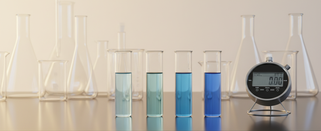
If doubling a reactant concentration makes a reaction four times faster, what does that tell you about its rate law? That one observation can reveal an experimentally determined reaction order. With a few carefully compared experiments, you can calculate the entire rate law, evaluate the rate constant k, and predict what happens when the starting concentrations change.
This college-level general chemistry guide explains the method of initial rates through an original four-experiment data set. You’ll derive the exponents, keep the units straight, and work through practice questions with answers.
Learning objectives
- Distinguish reaction rate, rate law, reaction order, and rate constant.
- Determine individual reaction orders from experimental ratios.
- Calculate a rate constant, including its correct units.
- Predict new initial rates from changes in reactant concentrations.
- Recognize how initial rate laws differ from integrated rate laws and balanced equations.
1. What does a chemical reaction rate measure?
Reaction rate describes how rapidly concentrations change with time. For a reaction aA → bB, a conventionally defined positive reaction rate is rate = −(1/a)(d[A]/dt) = (1/b)(d[B]/dt). Reactant concentration falls; product concentration rises. Stoichiometric coefficients connect the rates at which different species are consumed or produced.
This is different from the rate law, which describes how reaction rate depends on concentrations under a specified set of conditions. A general empirical form is rate = k[A]m[B]n. The exponents m and n are reaction orders and must ordinarily be determined from experiments.
Crucial exam distinction: you cannot usually read rate-law exponents from the balanced chemical equation. Only an established elementary step permits direct identification of the molecularity-based exponents from that step.
2. The experimental data: four initial-rate trials
Imagine an illustrative reaction involving reactants A and B. At one fixed temperature, the following invented teaching data were measured at the start of four runs. Each run changes the starting concentrations in a controlled way.
| Trial | Initial [A] (M) | Initial [B] (M) | Initial rate (M s−1) |
|---|---|---|---|
| 1 | 0.100 | 0.100 | 0.0200 |
| 2 | 0.200 | 0.100 | 0.0800 |
| 3 | 0.100 | 0.200 | 0.0400 |
| 4 | 0.200 | 0.200 | 0.160 |
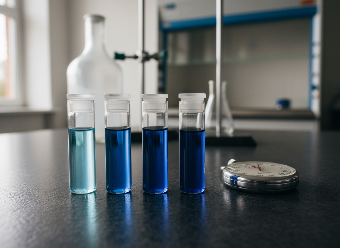
3. Determine the order with respect to A
Compare Trial 1 with Trial 2. The concentration of B stays at 0.100 M. A doubles from 0.100 M to 0.200 M, while the rate rises from 0.0200 to 0.0800 M/s—a factor of four.
For the unknown order m, the ratio is rate2/rate1 = ([A]2/[A]1)m, because k and [B] cancel. Thus 4 = 2m and m = 2.
The reaction is second order with respect to A. That does not imply two molecules of A necessarily collide in the single rate-determining event; an overall observed rate law may emerge from a multistep mechanism.
4. Determine the order with respect to B
Now compare Trial 1 with Trial 3. The starting concentration of A stays at 0.100 M, while B doubles. The measured rate doubles from 0.0200 to 0.0400 M/s.
By the same reasoning, 2 = 2n, so n = 1. The reaction is first order with respect to B.
5. Write the full experimentally determined rate law
Substitute the measured orders into the expression: rate = k[A]2[B]. The overall order is the sum of the exponents, 2 + 1 = 3. This is a third-order overall rate law.
Third order describes the concentration dependence, not the number of arrows in a balanced equation. If A doubles at constant B, rate multiplies by 22 = 4. If B doubles at constant A, rate multiplies by 2. If both double, rate multiplies by 4 × 2 = 8. Trial 4 verifies this prediction: 0.160/0.0200 = 8.
6. Find k and its units
Take the measurements from Trial 1 and solve for k: k = rate/([A]2[B]) = 0.0200 / ((0.100)2 × 0.100) = 20.0.
The units come from dimensional analysis. Rate has units M s−1, and [A]2[B] contributes M3. Therefore units of k = M−2 s−1. Our full answer is k = 20.0 M−2 s−1 for the chosen temperature.
| Overall order | Typical k units when rate is M/s |
|---|---|
| Zero | M s−1 |
| First | s−1 |
| Second | M−1 s−1 |
| Third | M−2 s−1 |
7. Use the rate law to make a new prediction
Problem: At the same temperature, a new mixture has [A] = 0.150 M and [B] = 0.200 M. Predict its initial rate.
Use the rate law with k = 20.0 M−2 s−1: rate = 20.0(0.150)2(0.200) = 0.0900 M s−1.
A shortcut is to compare this new mixture to Trial 1: A is multiplied by 1.50, and B by 2.00. Rate therefore changes by (1.50)2 × 2.00 = 4.50. Multiplying 0.0200 M/s by 4.50 again gives 0.0900 M/s.
8. Reaction order vs. integrated rate law
The method of initial rates answers how initial concentration affects the initial reaction rate. Integrated rate laws answer a different question: how does concentration change over time? For a separate first-order process, ln[A]t = ln[A]0 − kt and the half-life is t1/2 = ln 2/k.
For example, if a genuinely first-order process has k = 0.0231 min−1, its half-life is approximately 30.0 minutes. Do not apply this first-order half-life equation to our third-order rate-law example. Different overall orders require their own integrated treatments.
9. Temperature and catalysts: what changes?
For a given reaction over an appropriate temperature range, its rate constant often increases with temperature in a manner described by an Arrhenius-type equation: k = A0e−Ea/(RT). Here A0 is a pre-exponential factor, Ea is activation energy, R is the gas constant, and T is absolute temperature.
A catalyst may open a different kinetic pathway and increase reaction rate. It does not change the equilibrium constant at a fixed temperature. If your course covers equilibrium as well as kinetics, remember that how fast a mixture changes and where equilibrium lies are separate questions.
10. Five common errors and how to avoid them
- Reading exponents from coefficients: determine rate-law orders experimentally unless a true elementary step is specified.
- Comparing trials that change multiple concentrations: first choose pairs in which all but one concentration stay constant.
- Missing squared effects: doubling a second-order reactant multiplies rate by four, not two.
- Reporting k without units: calculate units from rate divided by the concentration product.
- Claiming a rate law proves a unique mechanism: several plausible mechanisms can sometimes yield the same observed rate law.
11. Practice problems
Problem A: For rate = 20.0[A]2[B], with the same units and conditions as the worked example, what happens to the rate when [A] is tripled and [B] is halved?
Problem B: For the same rate law, calculate the rate at [A] = 0.150 M and [B] = 0.200 M. Give appropriate units.
Problem C: A separate first-order reaction has k = 0.0231 min−1. Determine its half-life.
Problem D: For the balanced reaction 2 X → 3 Y, suppose d[X]/dt = −0.060 M s−1. What is the conventionally defined reaction rate, and how quickly is Y forming?
Practice answers with explanation
A: The factor is 32 × (1/2) = 4.50. The rate becomes 4.50 times the original, because A is second-order and B is first-order.
B: 0.0900 M s−1, from 20.0 × 0.1502 × 0.200. This repeats the worked prediction as a self-check.
C: t1/2 = 0.693/0.0231 = 30.0 min (three significant figures).
D: The reaction rate is −(1/2)(−0.060) = 0.030 M s−1. Since Y forms at three times the reaction rate, d[Y]/dt = +0.090 M s−1.
Reliable workflow: compare one changing variable, solve one exponent, repeat, determine k with units, then check the final data set.
Go deeper with trusted learning resources
For more examples of experimentally determined reaction orders, see OpenStax: Rate Laws. For time-dependent concentration equations, use OpenStax: Integrated Rate Laws. The PhET Reactions & Rates simulation provides a visual way to explore how reaction conditions affect collisions and rates. For another quantitative chemistry study guide, visit IntoChemistry’s stoichiometry tutorial.
Continue with free chemistry practice
Practice more rate-law problems and then try a mixed exam set. kinetics and rate-law lesson · General Chemistry exam practice.