
Calibration Graphs and Linear Regression
Turn measured calibration standards into a defensible equation and use it within the tested concentration range.
Fit a calibration line with ordinary least squares, solve for an unknown, and interpret residuals and R².
1. Arrange measured pairs
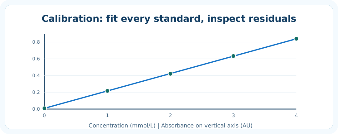
Plot known standard concentration x on the horizontal axis and measured analytical response y on the vertical axis. Include concentrations, units, instrument conditions, blank handling, and appropriate replicate information.
2. Fit the line
For ordinary least squares with an intercept, m=Σ[(x−x̄)(y−ȳ)]/Σ[(x−x̄)²] and b=ȳ−mx̄. Do not automatically force b=0 or calculate only from endpoints unless the method explicitly supports it.
3. Calculate an unknown
For y=mx+b, an unknown response yₓ corresponds to xₓ=(yₓ−b)/m. Use the unrounded regression coefficients. Check the unknown is inside the verified calibration range; dilute and remeasure otherwise.
4. Examine residuals
A residual is observed y minus fitted y. The scatter and pattern of residuals can reveal model problems. An R² close to 1 describes explained variation for those standards—not the accuracy of concentrations, absence of bias, or a validated dynamic range.
5. Document limitations
Include any replicate scatter, standard preparation uncertainty, blank effects, matrix effects, detector saturation, nonlinearity, and potential heteroscedasticity. Ordinary least squares is not automatically the right fit if errors vary greatly with concentration.
Quick understanding check
If a fitted line is y=0.050x+0.020 and a sample response is 0.270, what is x?
Reveal worked answer
x=(0.270−0.020)/0.050=5.00 in the units of the calibration x-axis.